Man and History

2023年2月14日星期二

Python 量子運算（二三）：外積

2023/02/10

-----

Fig. 23.1. Outer product.

-----

「Connection with the Kronecker product

The outer product and Kronecker product are closely related; in fact the same symbol is commonly used to denote both operations.

與克羅內克積的關係

外積與克羅內克積很接近；事實上，同一個符號通常用於表示這兩種操作。

」[1]。

-----

代碼 23.1

# Program 23.1：Outer product
import numpy as np
import matplotlib as mpl
import matplotlib.pyplot as plt


class Point:
    def __init__(self, x, y, z):
        self.x = x
        self.y = y
        self.z = z


def Line(ax, A, B):
    ax.plot([A.x, B.x], [A.y, B.y], [A.z, B.z], 'b')
    return


def Cube(ax, P1, P2):

    # parallel to x axis
    for z in range(P1.z, P2.z+1):
        S = Point(P1.x, P1.y, z)
        E = Point(P2.x, P1.y, z)
        Line(ax, S, E)
    for y in range(P1.y, P2.y+1):
        S = Point(P1.x, y, P2.z)
        E = Point(P2.x, y, P2.z)
        Line(ax, S, E)

    # parallel to y axis
    for x in range(P1.x, P2.x+1):
        S = Point(x, P1.y, P2.z)
        E = Point(x, P2.y, P2.z)
        Line(ax, S, E)
    for z in range(P1.z, P2.z+1):
        S = Point(P2.x, P1.y, z)
        E = Point(P2.x, P2.y, z)
        Line(ax, S, E)

    # parallel to z axis
    for x in range(P1.x, P2.x+1):
        S = Point(x, P1.y, P1.z)
        E = Point(x, P1.y, P2.z)
        Line(ax, S, E)
    for y in range(P1.y, P2.y+1):
        S = Point(P2.x, y, P1.z)
        E = Point(P2.x, y, P2.z)
        Line(ax, S, E)

    return


def Set(ax, lim):
    ax.set_xlim([0, lim])
    ax.set_ylim([0, lim])
    ax.set_zlim([0, lim])
    ax.set_axis_off()
    return


def Subplot_1():
    ax = plt.subplot(221)

    # string setting
    s1 = (
        r'$\mathbf{u} \otimes \mathbf{v} = \ $'
        r'$\mathbf{u} \mathbf{v}^{\operatorname{T}} =$'
    )
    s2 = (
        r'$\begin{bmatrix}$'
        r'$u_{1} \mathbf{v}^{\operatorname{T}} \\$'
        r'$\vdots \\$'
        r'$u_{m} \mathbf{v}^{\operatorname{T}}$'
        r'$\end{bmatrix}$'
    )

    # string output
    ax.text(0.1, 0.65, s1)
    ax.text(0.1, 0.35, s2)

    plt.title('Outer Product')
    ax.text(0.5, 0.05, '(a)', fontsize=20)
    ax.set_axis_off()

    return


def Subplot_2():
    ax = fig.add_subplot(222, projection='3d')  # 3d subplot

    P1 = Point(0, 0, 0)
    P2 = Point(1, 1, 3)
    Cube(ax, P1, P2)
    Set(ax, 6)

    for i in range(P2.z):
        for j in range(P2.x):
            ax.text(j, 0, i, r'$\mathbf{v}^{\operatorname{T}}$')

    plt.title('Rank 2 Tensor', color='r')
    ax.text(P2.x, P2.y, P2.z, r'matrix $(\mathbf{u} \otimes \mathbf{v})$')
    ax.text(4, 0, -1, '(b)', fontsize=20)

    return


def Subplot_3():
    ax = fig.add_subplot(223, projection='3d')  # 3d subplot

    P1 = Point(0, 0, 0)
    P2 = Point(1, 1, 3)
    Cube(ax, P1, P2)
    Set(ax, 6)

    plt.title('Rank 1 Tensor', color='r')
    ax.text(P2.x, P2.y, P2.z, r'vector $\mathbf{u}$')
    ax.text(4, 0, -1, '(c)', fontsize=20)

    return


def Subplot_4():
    ax = fig.add_subplot(224, projection='3d')  # 3d subplot

    P1 = Point(0, 0, 0)
    P2 = Point(4, 1, 1)
    Cube(ax, P1, P2)

    P3 = Point(5, 0, 0)
    P4 = Point(6, 1, 4)
    Cube(ax, P3, P4)

    Set(ax, 6)

    plt.title("Rank 1 Tensor", color='r')
    ax.text(0, 0, 3, 'Row Vecor(shape 1x4)', fontsize=16)
    ax.text(3, 0, 5, 'Column Vector(shape 4x1)', fontsize=16)
    ax.text(-1, 1, 1, r'vector $\mathbf{v}^{\operatorname{T}}$')
    ax.text(P4.x, P4.y, P4.z, r'vector $\mathbf{v}$')
    ax.text(4, 0, -1, '(d)', fontsize=20)

    return


# figure setting
mpl.rcParams['text.usetex'] = True
mpl.rcParams['text.latex.preamble'] = r'\usepackage{{amsmath}}'
mpl.rcParams['font.size'] = 40
fig = plt.figure(figsize=(16, 16))

Subplot_1()
Subplot_2()
Subplot_3()
Subplot_4()

plt.savefig('/content/drive/My Drive/pqc/0023_001.png')
# plt.show()

解說：

-----

References

[1] Outer product - Wikipedia

https://en.wikipedia.org/wiki/Outer_product

[2] NumPy Illustrated: The Visual Guide to NumPy | by Lev Maximov | Better Programming

https://en.wikipedia.org/wiki/Outer_product

[3] matplotlib - Python - Plotting colored grid based on values - Stack Overflow

https://stackoverflow.com/questions/43971138/python-plotting-colored-grid-based-on-values

-----

Python 量子運算（目錄）

https://mandhistory.blogspot.com/2022/01/quantum-computing.html

-----

Python 量子運算（二二）：克羅內克積

2023/02/09

-----

Fig. 22.1. Kronecker.

-----

目標是張量積，但進行之前，有必要先瞭解克羅內克積以及外積。

先看一下參考文獻一的結論：

外積是克羅內克積的特例 [2]。

對於向量而言，外積和是張量積等價的 [2]。

「In linear algebra, an outer product is the tensor product of two coordinate vectors, a special case of the Kronecker product of matrices.

在線性代數中，外積是兩個坐標向量的張量積，是矩陣的克羅內克積的特例。」[2]。

-----

代碼 22.1

# Program 22.1：Kronecker product
import numpy as np
import matplotlib as mpl
import matplotlib.pyplot as plt


class Point:
    def __init__(self, x, y, z):
        self.x = x
        self.y = y
        self.z = z


def Line(ax, A, B):
    ax.plot([A.x, B.x], [A.y, B.y], [A.z, B.z], 'b')
    return


def Cube(ax, P1, P2):

    # parallel to x axis
    for z in range(P1.z, P2.z+1):
        S = Point(P1.x, P1.y, z)
        E = Point(P2.x, P1.y, z)
        Line(ax, S, E)
    for y in range(P1.y, P2.y+1):
        S = Point(P1.x, y, P2.z)
        E = Point(P2.x, y, P2.z)
        Line(ax, S, E)

    # parallel to y axis
    for x in range(P1.x, P2.x+1):
        S = Point(x, P1.y, P2.z)
        E = Point(x, P2.y, P2.z)
        Line(ax, S, E)
    for z in range(P1.z, P2.z+1):
        S = Point(P2.x, P1.y, z)
        E = Point(P2.x, P2.y, z)
        Line(ax, S, E)

    # parallel to z axis
    for x in range(P1.x, P2.x+1):
        S = Point(x, P1.y, P1.z)
        E = Point(x, P1.y, P2.z)
        Line(ax, S, E)
    for y in range(P1.y, P2.y+1):
        S = Point(P2.x, y, P1.z)
        E = Point(P2.x, y, P2.z)
        Line(ax, S, E)

    return


def Set(ax, lim):
    ax.set_xlim([0, lim])
    ax.set_ylim([0, lim])
    ax.set_zlim([0, lim])
    ax.set_axis_off()
    return


def Subplot_1():
    ax = plt.subplot(221)

    # string setting
    s1 = r'$\mathbf{A} \otimes \mathbf{B} =$'
    s2 = (
        r'$\begin{bmatrix}$'
        r'$a_{11} \mathbf{B} & \cdots & a_{1n} \mathbf{B} \\$'
        r'$\vdots & \ddots & \vdots \\$'
        r'$a_{m1} \mathbf{B} & \cdots & a_{mn} \mathbf{B}$'
        r'$\end{bmatrix}$'
    )

    # string output
    ax.text(0.1, 0.65, s1)
    ax.text(0.1, 0.35, s2)

    plt.title('Kronecker Product')
    ax.text(0.5, 0.05, '(a)', fontsize=20)
    ax.set_axis_off()

    return


def Subplot_2():
    ax = fig.add_subplot(222, projection='3d')  # 3d subplot

    P1 = Point(0, 0, 0)
    P2 = Point(3, 1, 3)
    Cube(ax, P1, P2)
    Set(ax, 6)

    for i in range(P2.z):
        for j in range(P2.x):
            ax.text(j, 0, i, 'B')

    plt.title('Rank 2 Tensor', color='r')
    ax.text(P2.x, P2.y, P2.z, r'matrix $(\mathbf{A} \otimes \mathbf{B})$')
    ax.text(4, 0, -1, '(b)', fontsize=20)

    return


def Subplot_3():
    ax = fig.add_subplot(223, projection='3d')  # 3d subplot

    P1 = Point(0, 0, 0)
    P2 = Point(3, 1, 3)
    Cube(ax, P1, P2)
    Set(ax, 6)

    plt.title('Rank 2 Tensor', color='r')
    ax.text(P2.x, P2.y, P2.z, 'matrix A')
    ax.text(4, 0, -1, '(c)', fontsize=20)

    return


def Subplot_4():
    ax = fig.add_subplot(224, projection='3d')  # 3d subplot

    P1 = Point(0, 0, 0)
    P2 = Point(4, 1, 3)
    Cube(ax, P1, P2)
    Set(ax, 6)

    plt.title('Rank 2 Tensor', color='r')
    ax.text(P2.x, P2.y, P2.z, 'matrix B')
    ax.text(4, 0, -1, '(d)', fontsize=20)

    return


# figure setting
mpl.rcParams['text.usetex'] = True
mpl.rcParams['text.latex.preamble'] = r'\usepackage{{amsmath}}'
mpl.rcParams['font.size'] = 40
fig = plt.figure(figsize=(16, 16))

Subplot_1()
Subplot_2()
Subplot_3()
Subplot_4()

# plt.savefig('/content/drive/My Drive/pqc/0022_001.png')
plt.show()

解說：

-----

References

[1] Kronecker product - Wikipedia

https://en.wikipedia.org/wiki/Kronecker_product

[2] 淺談張量分解（四）：外積、Kronecker積和張量積- 知乎

https://zhuanlan.zhihu.com/p/26774182

[3] 8 ways to use the Kronecker product - The DO Loop

https://blogs.sas.com/content/iml/2020/07/27/8-ways-kronecker-product.html

[4] numpy.kron — NumPy v1.24 Manual

https://numpy.org/doc/stable/reference/generated/numpy.kron.html

# 矩陣

[5] 使用說明:數學公式 - 維基教科書，自由的教學讀本

https://zh.wikibooks.org/zh-tw/Help:%E6%95%B0%E5%AD%A6%E5%85%AC%E5%BC%8F

# 字串太長

[6] Python 慣用語 - 8 太長怎麼辦 « Python Life

http://seanlin.logdown.com/posts/210861-python-idioms-8-too-long

-----

Python 量子運算（目錄）

https://mandhistory.blogspot.com/2022/01/quantum-computing.html

-----

Python 量子運算（二一）：張量

2023/02/19

-----

Fig. 21.1. Tensor.

-----

純量：秩 0 的張量。

向量：秩 1 的張量。

矩陣：秩 2 的張量。

張量：秩 3 及以上稱為張量。

-----

代碼 21.1

# Program 21.1：Tensor
import numpy as np
import matplotlib as mpl
import matplotlib.pyplot as plt


class Point:
    def __init__(self, x, y, z):
        self.x = x
        self.y = y
        self.z = z


def Line(ax, A, B):
    ax.plot([A.x, B.x], [A.y, B.y], [A.z, B.z], 'b')
    return


def Cube(ax, P1, P2):

    # parallel to x axis
    for z in range(P1.z, P2.z+1):
        S = Point(P1.x, P1.y, z)
        E = Point(P2.x, P1.y, z)
        Line(ax, S, E)
    for y in range(P1.y, P2.y+1):
        S = Point(P1.x, y, P2.z)
        E = Point(P2.x, y, P2.z)
        Line(ax, S, E)

    # parallel to y axis
    for x in range(P1.x, P2.x+1):
        S = Point(x, P1.y, P2.z)
        E = Point(x, P2.y, P2.z)
        Line(ax, S, E)
    for z in range(P1.z, P2.z+1):
        S = Point(P2.x, P1.y, z)
        E = Point(P2.x, P2.y, z)
        Line(ax, S, E)

    # parallel to z axis
    for x in range(P1.x, P2.x+1):
        S = Point(x, P1.y, P1.z)
        E = Point(x, P1.y, P2.z)
        Line(ax, S, E)
    for y in range(P1.y, P2.y+1):
        S = Point(P2.x, y, P1.z)
        E = Point(P2.x, y, P2.z)
        Line(ax, S, E)

    return


def Set(ax, lim):
    ax.set_xlim([0, lim])
    ax.set_ylim([0, lim])
    ax.set_zlim([0, lim])
    ax.set_axis_off()
    return


def Subplot_1():
    ax = fig.add_subplot(221, projection='3d')  # 3d subplot

    P1 = Point(0, 0, 0)
    P2 = Point(1, 1, 1)
    Cube(ax, P1, P2)
    Set(ax, 6)

    plt.title('Rank 0 Tensor', color='r')
    ax.text(P2.x, P2.y, P2.z, 'scalar')
    ax.text(4, 0, -1, '(a)', fontsize=20)

    return


def Subplot_2():
    ax = fig.add_subplot(222, projection='3d')  # 3d subplot

    P1 = Point(0, 0, 0)
    P2 = Point(4, 1, 1)
    Cube(ax, P1, P2)

    P3 = Point(5, 0, 0)
    P4 = Point(6, 1, 3)
    Cube(ax, P3, P4)

    Set(ax, 6)

    plt.title("Rank 1 Tensor", color='r')
    ax.text(0, 0, 3, 'Row Vecor(shape 1x4)', fontsize=16)
    ax.text(3, 0, 5, 'Column Vector(shape 3x1)', fontsize=16)
    ax.text(P4.x, P4.y, P4.z, 'vector')
    ax.text(4, 0, -1, '(b)', fontsize=20)

    return


def Subplot_3():
    ax = fig.add_subplot(223, projection='3d')  # 3d subplot

    P1 = Point(0, 0, 0)
    P2 = Point(4, 1, 3)
    Cube(ax, P1, P2)
    Set(ax, 6)

    plt.title('Rank 2 Tensor', color='r')
    ax.text(P2.x, P2.y, P2.z, 'matrix')
    ax.text(4, 0, -1, '(c)', fontsize=20)

    return


def Subplot_4():
    ax = fig.add_subplot(224, projection='3d')  # 3d subplot

    P1 = Point(0, 0, 0)
    P2 = Point(4, 5, 3)
    Cube(ax, P1, P2)
    Set(ax, 6)

    plt.title('Rank 3 Tensor', color='r')
    ax.text(P2.x, P2.y, P2.z, 'tensor')
    ax.text(4, 0, -1, '(d)', fontsize=20)

    return


# figure setting
mpl.rcParams['font.size'] = 40
fig = plt.figure(figsize=(16, 16))

Subplot_1()
Subplot_2()
Subplot_3()
Subplot_4()

# plt.savefig('/content/drive/My Drive/pqc/0021_001.png')
plt.show()

解說：

-----

References

[1] 淺談張量分解（一）：如何簡單地進行張量分解？ - 知乎

https://zhuanlan.zhihu.com/p/24798389

[2] 淺談張量分解（二）：張量分解的數學基礎- 知乎

https://zhuanlan.zhihu.com/p/24824550

[3] 淺談張量分解（三）：如何對稀疏矩陣進行奇異值分解？ - 知乎

https://zhuanlan.zhihu.com/p/25512080

[4] 淺談張量分解（四）：外積、Kronecker積和張量積- 知乎

https://zhuanlan.zhihu.com/p/26774182

[5] 淺談張量分解（五）：稀疏張量的CP分解- 知乎

https://zhuanlan.zhihu.com/p/25067269

# 張量

[6] Tensor Explained with Python Numpy Examples - Data Analytics

https://vitalflux.com/tensor-explained-with-python-numpy-examples/

# 張量

[7] TensorFlow ranks and tensors | Python Machine Learning - Second Edition

https://subscription.packtpub.com/book/big-data-and-business-intelligence/9781787125933/14/ch14lvl1sec85/tensorflow-ranks-and-tensors

# 向量的矩陣

[8] What is a Tensor? | Medium

https://furkangulsen.medium.com/what-is-a-tensor-ce8e78835d08

# 矩陣的向量

[9] Chapter 1. Tensor — TensorFlow.NET 0.6.0 documentation

https://tensorflownet.readthedocs.io/en/latest/Tensor.html

# 張量

[10] What is the Tensor in deep learning? | by Bala Venkatesh | DataDrivenInvestor

https://medium.datadriveninvestor.com/what-is-the-tensor-in-deep-learning-77c2af7224a1

# 繪圖

[11] Appendix: Figure Code | Python Data Science Handbook

https://jakevdp.github.io/PythonDataScienceHandbook/06.00-figure-code.html

-----

Python 量子運算（目錄）

https://mandhistory.blogspot.com/2022/01/quantum-computing.html

-----

2023年2月9日星期四

Python 量子運算（二０）：叉積範例

2023/02/08

-----

Fig. 20.1. Cross product examples.

-----

代碼 20.1

# Program 20.1：Cross product examples
import numpy as np
import matplotlib as mpl
import matplotlib.pyplot as plt
from matplotlib.ticker import MaxNLocator


# type 1: defined by angle
class VectorT1:
    def __init__(self, r, p):
        self.r = r  # radius
        self.p = p  # phi

        self.x = 0
        self.y = 0
        self.z = 0

        self.u = r * np.cos(p)
        self.v = r * np.sin(p)
        self.w = 0


# type 2:defined by points
class VectorT2:
    def __init__(self, u, v, w):
        self.x = 0
        self.y = 0
        self.z = 0

        self.u = u
        self.v = v
        self.w = w


def Subplot(i, j):
    n = i * 3 + j + 1
    if n == 5:
        return
    ax = fig.add_subplot(3, 3, n, projection='3d')  # 3d subplot

    # vector blue
    vb_r = 2
    vb_p = 0
    vb = VectorT1(vb_r, vb_p)

    p = [3, 2, 1, 4, 0, 0, 5, 6, 7]
    # title = ['135', '90', '45', '180', '0', '0', '225', '270', '315']
    title = [r"$135^{\circ}$", r"$90^{\circ}$", r"$45^{\circ}$",
             r"$180^{\circ}$", '0', r"$0^{\circ}$",
             r"$135^{\circ}$", r"$90^{\circ}$", r"$45^{\circ}$"]

    # vector red
    vr_r = 2
    vr_p = (p[n - 1] / 8) * 2 * np.pi
    vr = VectorT1(vr_r, vr_p)
    plt.title(title[n - 1], fontsize=40)

    # vector purple
    op = vb.r * vr.r * np.sin(vr.p-vb.p)
    vp = VectorT2(0, 0, op)

    ax.quiver(vb.x, vb.y, vb.z, vb.u, vb.v, vb.w, color='b')
    ax.quiver(vr.x, vr.y, vr.z, vr.u, vr.v, vr.w, color='r')
    ax.quiver(vp.x, vp.y, vp.z, vp.u, vp.v, vp.w, color='purple')

    # arc phi
    if vr.p < np.pi:
        phi = np.linspace(0, vr.p-vb.p, 100)
    elif vr.p > np.pi:
        phi = np.linspace(vr.p-vb.p, 2*np.pi, 100)
    else:
        phi = np.linspace(0, 0, 100)
    x2 = 1 * np.cos(phi)
    y2 = 1 * np.sin(phi)
    ax.plot(x2, y2, 'k')

    ax.set_xlim([-5, 5])
    ax.set_ylim([-5, 5])
    ax.set_zlim([-5, 5])
    ax.xaxis.set_major_locator(MaxNLocator(3))
    ax.yaxis.set_major_locator(MaxNLocator(3))
    ax.zaxis.set_major_locator(MaxNLocator(3)) 

    return


# figure setting
mpl.rcParams['text.usetex'] = True
mpl.rcParams['text.latex.preamble'] = r'\usepackage{{amsmath}}'
mpl.rcParams['font.size'] = 16
fig = plt.figure(figsize=(16, 16))

for i in range(3):
    for j in range(3):
        Subplot(i, j)

# plt.savefig('/content/drive/My Drive/pqc/0020_001.png')
plt.show()

解說：

此代碼以繪出向量外積為目的，方便為主，並未嚴格按照外積的公式。

-----

References

[1] 外積 - 維基百科，自由的百科全書

https://zh.wikipedia.org/zh-tw/%E5%8F%89%E7%A7%AF

[2] 在 Matplotlib 中設定 Ticks 刻度數量 | D棧 - Delft Stack

https://www.delftstack.com/zh-tw/howto/matplotlib/matplotlib-set-number-of-ticks/

-----

Python 量子運算（目錄）

https://mandhistory.blogspot.com/2022/01/quantum-computing.html

-----

Python 量子運算（一九）：叉積

2023/02/06

-----

Fig. 19.1 Cross product.

-----

代碼 19.1

# Program 19.1：Cross product
import numpy as np
import matplotlib as mpl
import matplotlib.pyplot as plt


# type 1: defined by angle
class VectorT1:
    def __init__(self, r, p):
        self.r = r  # radius
        self.p = p  # phi

        self.x = 0
        self.y = 0
        self.z = 0

        self.u = r * np.cos(p)
        self.v = r * np.sin(p)
        self.w = 0


# type 2:defined by points
class VectorT2:
    def __init__(self, u, v, w):
        self.x = 0
        self.y = 0
        self.z = 0

        self.u = u
        self.v = v
        self.w = w


# figure setting
mpl.rcParams['text.usetex'] = True
mpl.rcParams['text.latex.preamble'] = r'\usepackage{{amsmath}}'
mpl.rcParams['font.size'] = 40
fig = plt.figure(figsize=(16, 16))
ax = fig.add_subplot(111, projection='3d')  # 3d subplot

# vector blue
vb_r = 2
vb_p = 0
vb = VectorT1(vb_r, vb_p)

# vector red
vr_r = 2
vr_p = (1/3) * np.pi
vr = VectorT1(vr_r, vr_p)

# vector purple
op = vb.r * vr.r * np.sin(vr.p-vb.p)
vp = VectorT2(0, 0, op)

# vector grey
vg = VectorT2(0, 0, 1)

ax.quiver(vb.x, vb.y, vb.z, vb.u, vb.v, vb.w, color='b', linewidth=5)
ax.quiver(vr.x, vr.y, vr.z, vr.u, vr.v, vr.w, color='r', linewidth=5)
ax.quiver(vp.x, vp.y, vp.z, vp.u, vp.v, vp.w, color='purple', linewidth=5)
ax.quiver(vg.x, vg.y, vg.z, vg.u, vg.v, vg.w, color='grey', linewidth=8)

# arc phi
phi = np.linspace(0, vr.p-vb.p, 100)
x2 = 0.5 * np.cos(phi)
y2 = 0.5 * np.sin(phi)
ax.plot(x2, y2, 'k')

ax.set_xlim([0, 4])
ax.set_ylim([0, 4])
ax.set_zlim([0, 4])

s1 = r'$\mathbf{a}=(2,0,0)$'
s2 = r'$\mathbf{b}=(1,\sqrt3,0)$'
s3 = r'$\mathbf{a}\times\mathbf{b}'\
     r'=\|\mathbf{a}\|\|\mathbf{b}\| \sin(\phi)\mathbf{\hat n}=(0,0,2\sqrt3)$'
s4 = r'$\mathbf{\hat n}=(0,0,1)$'
s5 = r'$\phi=60^{\circ}$'

ax.text(vb.u+0.3, vb.v, vb.w, s1, color='b')
ax.text(vr.u+0.3, vr.v, vr.w, s2, color='r')
ax.text(vp.u+0.3, vp.v, vp.w, s3, color='purple')
ax.text(vg.u+0.3, vg.v, vg.w, s4, color='grey')
ax.text(vb.x+0.6, vb.y+0.2, vb.z, s5, color='k')

# plt.savefig('/content/drive/My Drive/pqc/0019_001.png')
plt.show()

解說：

此代碼以繪出向量外積為目的，方便為主，並未嚴格按照外積的公式。

-----

References

[1] Cross product - Wikipedia

https://en.wikipedia.org/wiki/Cross_product

[2] Unit vector - Wikipedia

https://en.wikipedia.org/wiki/Unit_vector

[3] Polar coordinate system - Wikipedia

https://en.wikipedia.org/wiki/Polar_coordinate_system

[4] matplotlib.pyplot.quiver — Matplotlib 3.6.2 documentation

https://matplotlib.org/stable/api/_as_gen/matplotlib.pyplot.quiver.html

[5] 3D quiver plot — Matplotlib 3.6.3 documentation

https://matplotlib.org/stable/gallery/mplot3d/quiver3d.html

[6] Python Matplotlib: How to draw 3D vector - OneLinerHub

https://onelinerhub.com/python-matplotlib/how-to-draw-3d-vector

-----

Python 量子運算（目錄）

https://mandhistory.blogspot.com/2022/01/quantum-computing.html

-----

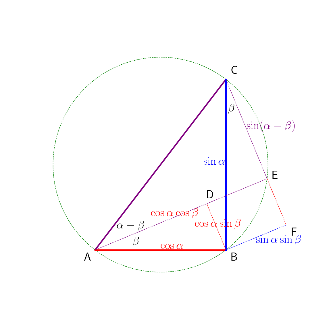
Python 量子運算（一七）：差角

2023/02/01

-----

Fig. 17. 1 Angle difference.

-----

代碼 17.1

# Program 17.1：Angle difference
import numpy as np
import matplotlib as mpl
import matplotlib.pyplot as plt


# defined by angle
class PointT1:
    def __init__(self, t, r):
        self.t = t  # theta

        self.r = r  # radius
        self.x = r * np.cos(t)
        self.y = r * np.sin(t)


# defined by points
class PointT2:
    def __init__(self, x, y):
        self.x = x
        self.y = y


def Subplot_1():
    ax = plt.subplot(111)

    # circle
    c = np.linspace(0, np.pi*2, 100)
    r = 1
    c_x = r * np.cos(c)
    c_y = r * np.sin(c)
    ax.plot(c_x, c_y, 'g', linestyle='--')

    t_A = (31/24) * np.pi                # theta A setting
    PA = PointT1(t_A, r)                 # A
    PC = PointT1(t_A-np.pi, r)           # C, determined by A
    ax.plot([PA.x, PC.x], [PA.y, PC.y])  # AC
    ax.plot([PA.x, PC.x], [PA.y, PC.y], 'purple', linewidth=5.0)  # AC
    ax.text(PA.x-0.1, PA.y-0.1, 'A')
    ax.text(PC.x+0.05, PC.y+0.05, 'C')

    PB = PointT2(PC.x, PA.y)             # B, determined by A, C
    ax.plot([PA.x, PB.x], [PA.y, PA.y])  # AB
    ax.plot([PB.x, PB.x], [PB.y, PC.y])  # BC
    ax.plot([PA.x, PB.x], [PA.y, PA.y], 'r', linewidth=5.0)  # AB
    ax.plot([PB.x, PB.x], [PB.y, PC.y], 'b', linewidth=5.0)  # BC
    ax.text(PB.x+0.05, PB.y-0.1, 'B')

    t_E = (47/24) * np.pi                # theta E setting
    PE = PointT1(t_E, r)                 # E
    ax.plot([PA.x, PE.x], [PA.y, PE.y], 'purple', linestyle='--')  # AE
    ax.plot([PC.x, PE.x], [PC.y, PE.y], 'purple', linestyle='--')  # CE
    ax.text(PE.x+0.05, PE.y, 'E')

    # finding Point G for learning
    slope_AE = (PE.y - PA.y) / (PE.x - PA.x)
    # PG_x = PB.x
    # PG_y = (PG_x - PA.x) * slope_AE + PA.y
    # PG = PointT2(PG_x, PG_y)
    # ax.plot([PB.x, PG.x], [PB.y, PG.y], 'k')  # BG

    # finding Point D
    slope_CE = (PE.y - PC.y) / (PE.x - PC.x)  # -(1/slope_AE)
    slope_BD = slope_CE
    # (PD_y - PA.y) / (PD_x - PA.x) = slope_AE
    # (PD_y - PB.y) / (PD_x - PB.x) = slope_BD
    # (PD_y) = slope_AE * (PD_x - PA.x) + PA.y
    # (PD_y) = slope_BD * (PD_x - PB.x) + PB.y
    # slope_AE * (PD_x - PA.x) + PA.y = slope_BD * (PD_x - PB.x) + PB.y
    x1 = (slope_AE * PA.x - slope_BD * PB.x + PB.y - PA.y)
    x2 = (slope_AE - slope_BD)
    PD_x = x1 / x2

    # PH = PointT2(PD_x, PA.y)                  # for verifying PD_x
    # ax.plot([PB.x, PH.x], [PB.y, PH.y], 'k')  # for verifying PD_x

    PD_y = slope_AE * (PD_x - PA.x) + PA.y
    PD = PointT2(PD_x, PD_y)
    ax.plot([PB.x, PD.x], [PB.y, PD.y], 'r', linestyle='--')  # BD
    ax.text(PD.x, PD.y+0.05, 'D')

    # finding Point F
    PF_x = PE.x - PD.x + PB.x
    PF_y = PE.y - PD.y + PB.y
    PF = PointT2(PF_x, PF_y)
    ax.plot([PB.x, PF.x], [PB.y, PF.y], 'b', linestyle='--')  # BF
    ax.plot([PE.x, PF.x], [PE.y, PF.y], 'r', linestyle='--')  # EF
    ax.text(PF.x+0.05, PF.y-0.1, 'F')

    # angles
    ax.text(PA.x+0.20, PA.y+0.20, r'$\alpha-\beta$')
    ax.text(PA.x+0.35, PA.y+0.05, r'$\beta$')
    ax.text(PC.x+0.02, PC.y-0.30, r'$\beta$')

    # edges
    ax.text((PA.x+PB.x)/2, (PA.y+PB.y)/2+0.01,
            r'$\cos\alpha$', color='r')
    ax.text((PA.x+PD.x)/2, (PA.y+PD.y)/2+0.10,
            r'$\cos\alpha\cos\beta$', color='r')
    ax.text((PB.x+PD.x)/2-0.20, (PB.y+PD.y)/2,
            r'$\cos\alpha\sin\beta$', color='r')

    ax.text((PB.x+PC.x)/2-0.21, (PB.y+PC.y)/2,
            r'$\sin\alpha$', color='b')
    ax.text((PB.x+PF.x)/2, (PB.y+PF.y)/2-0.05,
            r'$\sin\alpha\sin\beta$', color='b')

    ax.text((PC.x+PE.x)/2, (PC.y+PE.y)/2,
            r'$\sin(\alpha-\beta)$', color='purple')

    ax.set_aspect(1)  # height : width
    ax.set_axis_off()

    return


mpl.rcParams['text.usetex'] = True
mpl.rcParams['text.latex.preamble'] = r'\usepackage{{amsmath}}'
mpl.rcParams['font.size'] = 40
fig = plt.figure(figsize=(16, 16))

Subplot_1()

# plt.savefig('/content/drive/My Drive/pqc/0017_001.png')
plt.show()

解說：

-----

訂閱：文章 (Atom)

2023年2月14日 星期二

Python 量子運算（二三）：外積

Python 量子運算（二二）：克羅內克積

Python 量子運算（二一）：張量

2023年2月9日 星期四

Python 量子運算（二０）：叉積範例

Python 量子運算（一九）：叉積

Python 量子運算（一七）：差角

2023年2月14日星期二

2023年2月9日星期四