Python 量子運算(三0):直角坐標系與和角
2023/02/26
-----

Fig. 30.1. Cartesian coordinate system and angle sum.
-----
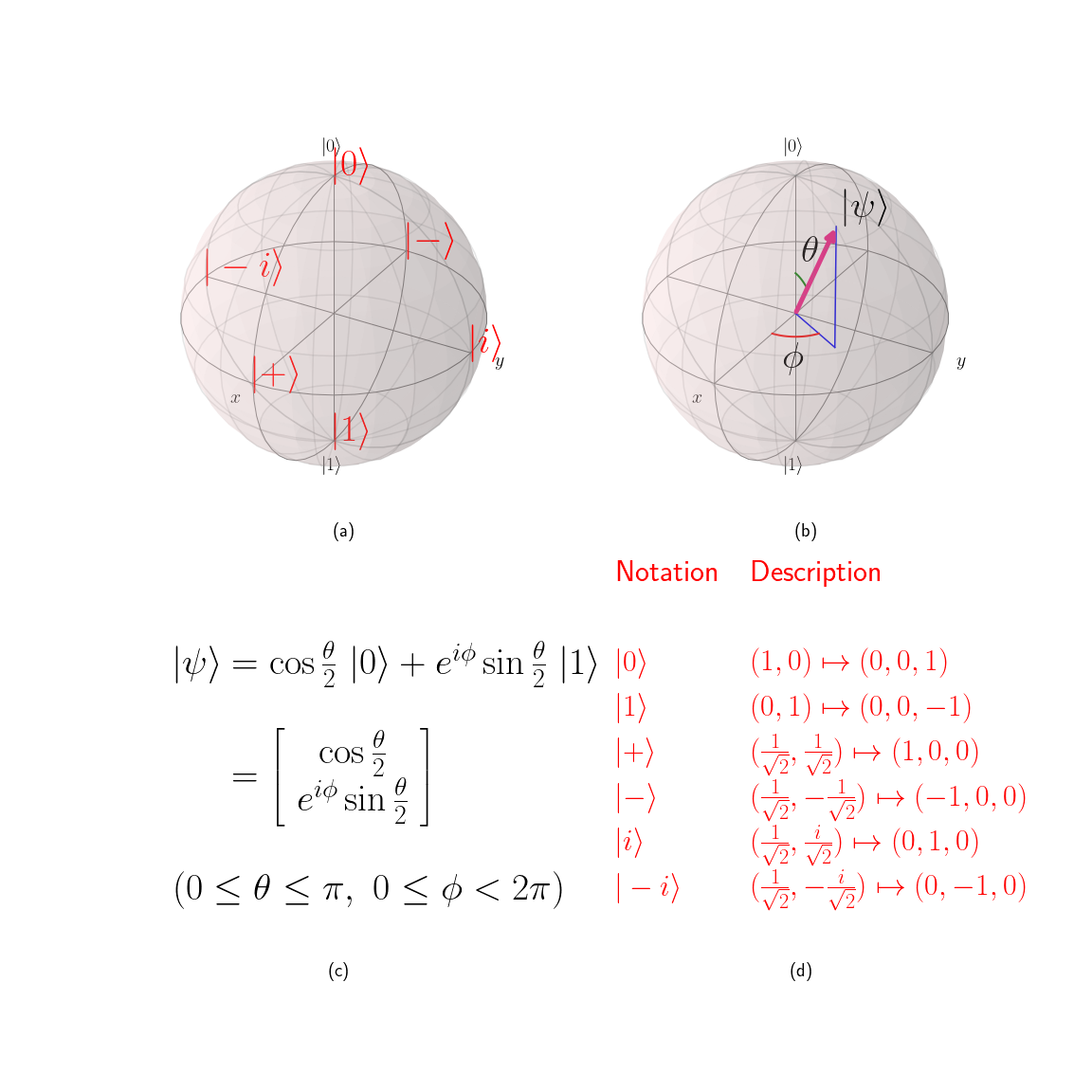
1 2 3 4 5 6 7 8 9 10 11 12 13 14 15 16 17 18 19 20 21 22 23 24 25 26 27 28 29 30 31 32 33 34 35 36 37 38 39 40 41 42 43 44 45 46 47 48 49 50 51 52 53 54 55 56 57 58 59 60 61 62 63 64 65 66 67 68 69 70 71 72 73 74 75 76 77 78 79 80 81 82 83 84 85 86 87 88 89 90 91 92 93 94 95 96 97 98 99 100 101 102 103 104 105 106 107 108 109 110 111 112 113 114 115 116 117 118 119 120 121 122 123 124 125 126 127 128 129 130 131 132 | # Program 30.1:Cartesian coordinate system and angle sum import matplotlib as mpl import matplotlib.pyplot as plt from qiskit.visualization import plot_bloch_vector def Subplot_1(): ax = plt.subplot(221) s1 = ( r'$\vert 0 \rangle \equiv $' r'$\begin{bmatrix} 1 \\ 0 \end{bmatrix} \mapsto (0,0,1)$' ) s2 = ( r'$\vert 1 \rangle \equiv $' r'$\begin{bmatrix} 0 \\ 1 \end{bmatrix} \mapsto (0,0,-1)$' ) s3 = r'$\psi_x=\cos \phi \sin \theta$' s4 = r'$\psi_y=\sin \phi \sin \theta$' s5 = r'$\psi_z=\cos \theta$' ax.text(0.15, 0.90, s1) ax.text(0.15, 0.60, s2) ax.text(0.15, 0.30, s3, color='r') ax.text(0.15, 0.20, s4, color='r') ax.text(0.15, 0.10, s5, color='r') ax.text(0.5, -0.055, '(a)', fontsize=20) ax.set_axis_off() return def Subplot_2(): ax = plt.subplot(222) # string setting s1_1 = r'$\sin(\alpha+\beta)$' s1_2 = r'$=\sin\alpha\cos\beta+\cos\alpha\sin\beta$' s1_3 = r'$\sin \theta = 2 \sin \frac{\theta}{2} \cos \frac{\theta}{2}$' s2_1 = r'$\cos(\alpha+\beta)$' s2_2 = r'$=\cos\alpha\cos\beta-\sin\alpha\sin\beta$' s2_3 = r'$\cos \theta = \cos^2 \frac{\theta}{2} - \sin^2 \frac{\theta}{2}$' # string output ax.text(0.10, 0.95, s1_1) ax.text(0.20, 0.80, s1_2) ax.text(0.10, 0.65, s1_3, color='r') ax.text(0.20, 0.45, s2_1) ax.text(0.10, 0.30, s2_2) ax.text(0.10, 0.15, s2_3, color='r') ax.text(0.5, -0.055, '(b)', fontsize=20) ax.set_axis_off() return def Subplot_3(): ax = plt.subplot(223) # string setting s1_1 = r'$\vert\psi\rangle$' s1_2 = ( r'$=\cos\frac{\theta}{2}\ \vert0\rangle' r'+e^{i\phi}\sin\frac{\theta}{2}\ \vert1\rangle$' ) s2 = ( r'$=\begin{bmatrix}\cos\frac{\theta}{2}\\$' r'$\ e^{i\phi}\sin\frac{\theta}{2}\ \end{bmatrix}$' ) s3 = r'$(0\leq\theta\leq\pi,\ 0\leq\phi<2\pi)$' # string output ax.text(0.10, 0.75, s1_1) ax.text(0.25, 0.75, s1_2) ax.text(0.25, 0.45, s2) ax.text(0.10, 0.15, s3) ax.text(0.5, -0.055, '(c)', fontsize=20) ax.set_axis_off() return def Subplot_4(): ax = plt.subplot(224) # string setting s1 = r'$1 = \cos^2 \frac{\theta}{2} + \sin^2 \frac{\theta}{2}$' s2 = r'$e ^{i\phi} = \cos \phi + i \sin \phi$' s3 = ( r'$\vert \psi \rangle =\ $' r'$\begin{bmatrix}$' r'$\sqrt \frac{1+\psi_z}{2} \\$' r'$\frac{\psi_x+i\psi_y}{\sqrt{2(1+\psi_z)}}$' r'$\end{bmatrix}$' ) # string output ax.text(0.10, 0.95, s1, color='r') ax.text(0.10, 0.85, s2, color='r') ax.text(0.10, 0.35, s3, color='r', fontsize=70) ax.text(0.5, -0.055, '(d)', fontsize=20) ax.set_axis_off() return # figure setting mpl.rcParams['text.usetex'] = True mpl.rcParams['text.latex.preamble'] = r'\usepackage{{amsmath}}' mpl.rcParams['font.size'] = 40 fig, ax = plt.subplots(figsize=(16, 16)) Subplot_1() Subplot_2() Subplot_3() Subplot_4() # plt.savefig('/content/drive/My Drive/pqc/0030_001.png', facecolor='w') plt.show() |
-----
References
-----
Python 量子運算(目錄)
https://mandhistory.blogspot.com/2022/01/quantum-computing.html
-----